Algorithms regarding to Trees
Trees is one of the greatest areas in graph theory covered in informatics contests, and is increasing in popularity rapidly. In this blog we cover some tree algorithms.
Notes
- Let $\mathcal{T}$ denote a Tree
- Familiarity is assumed with fundamental algorithms of trees like LCA and important principles like Euler tour and diameter.
Two Lemmas on the diameter
- If node sets $X$ and $Y$ are diameters of a tree, then $X\cap Y\neq \emptyset$.
- For any node $v\in \mathcal{T}$, the furthest node $u$ from $v$ is the endpoint of at least 1 diameter path.
We Prove these lemmas Here.
Proof (1):
We proceed constructively. Consider a midpoint of one of the diameters X (i.e a middle node in the path). If this midpoint is not also a midpoint of the other diameter then we can form a longer path by connecting one of the halves of X to a part of Y. We leave the details to the reader. This midpoint is called the centre.
Proof (2): Suppose $A,B$ are the endpoint of a diameter and WLOG $d(v,A)\leq d(v,B)\leq d(v,u)$. Rooting the tree at $v$, consider $C$ the lowest common ancestor LCA of $B$ and $u$. Then $d(C,B)\leq d(c,u)$ by assumption that $u$ is the furtherest node. If the path $UV$ is disjoint from $AB$ then $d(A,u) = d(A,c) + d(c,u) \geq d(A,B)$ so $u$ is also the endpoint of a diameter. If the paths share an edge the logic also falls out similarly.
Applications of the two lemmas.
Arguably, Lemma 2 is the more useful of the two. Lets consider two problems.
Problem 1 Module task: Given hidden tree of N nodes, you can query distance between two points. Find the length of the diameter in 2N queries.
Answer: Trivial application of lemma 2.
Problem 2 Given unweighted tree construct permutation of nodes $v_1 … v_N$ such that $d(v_i,v_{i+1})\geq d(v_{i+1}, v_{i+2})$.
Answer: Lets find a diameter of a tree and let its endpoint be $x$. We construct the sequence by repeatedly finding the furtherest node from $x$. Observe that at each iteration of the algorithm the diameter of the tree is nonincreasing. Further, we prove inductively that at each iteration the node we currently occupy is an endpoint of at least 1 diameter on the tree. Lets suppose that from $x$ we go to $y$. Then $xy$ is a diameter path clearly by definition. Now from $y$ we can at least guarantee a diameter of $d(x,y)-1$ by going from $y$ to the second node in the path from $x$ to $y$. If there still exist a path of length $d(x,y)$ then it must share an node with the path $xy$ by Lemma 1. As such when the tree is rerooted at $y$ the endpoints of the previous diameter become accessible to $y$ and we will jump to there instead.
Problems to ponder:
- APIO 2020 Fun tour
- IOI 2015 Towns
Centres of the Tree
There are several important points in every tree
Centroid: This node minimises the sum of distances to every other node in the tree, and also has many other useful properties
Centre of tree: Minimises the depth of the tree if rooted at it. Found by taking the midpoint of the diameter. A tree has one or two centres.
We will not in depth cover the Centre, but focus on Centroid.
Property of Centroid: In addition to minimising the sum of distances, the centroid splits the tree into subtrees, none of which have more nodes than half the side of the tree.
Proof: Suppose otherwise, then if we shift the centroid towards subtree with the majority of the nodes then we reduce distance sum. We can use this of thus construct the centroid by starting at a leaf and repeatedly walking in a direction that minimises distance sum.
Applications: The main application for centroids is centroid decomposition. Effectively, we find the centroid, remove it and recursively apply the process onto the resulting subtrees. It is equivalent to divide and conquer on tree, and facilitates many effective algorithms for interactive and data structure problems.
Example: Maintain weighted tree with edge updates, after each update find diameter length.
Solution: Consider the set of trees $\mathcal{S}$ produced by the centroid decomposition (i.e the original tree, the trees produced by the deletion of the first centroid, the second, etc). The total size of these trees is $O(NlogN)$ by the divide and conquer procedure. In this procedure, the intact diameter path must pass through the centroid of at least one of these trees. Thus by rooting each of the trees in $\mathcal{S}$ at the centroid of each tree, we only need to consider the paths passing through the root of each centroid tree and take the maximum overall. This can be maintained with lazy proprogation segment tree. When updates happen, we update the centroid trees of the $O(logN)$ centroid trees containing that edge.
This demonstrates the key idea of centroid decomposition, that every path passes through a centroid in some centroid tree. Centroid decomposition has other applications too, such as:
- Binary search on Tree
- Setting up a tree for pairing style problems where a majority is undesirable
Problems to ponder
- Dynamic Diameter (CEOI20)
- JOI2020 Capital City
Virtual Tree
The whole concept of virtual tree centres around the following fact:
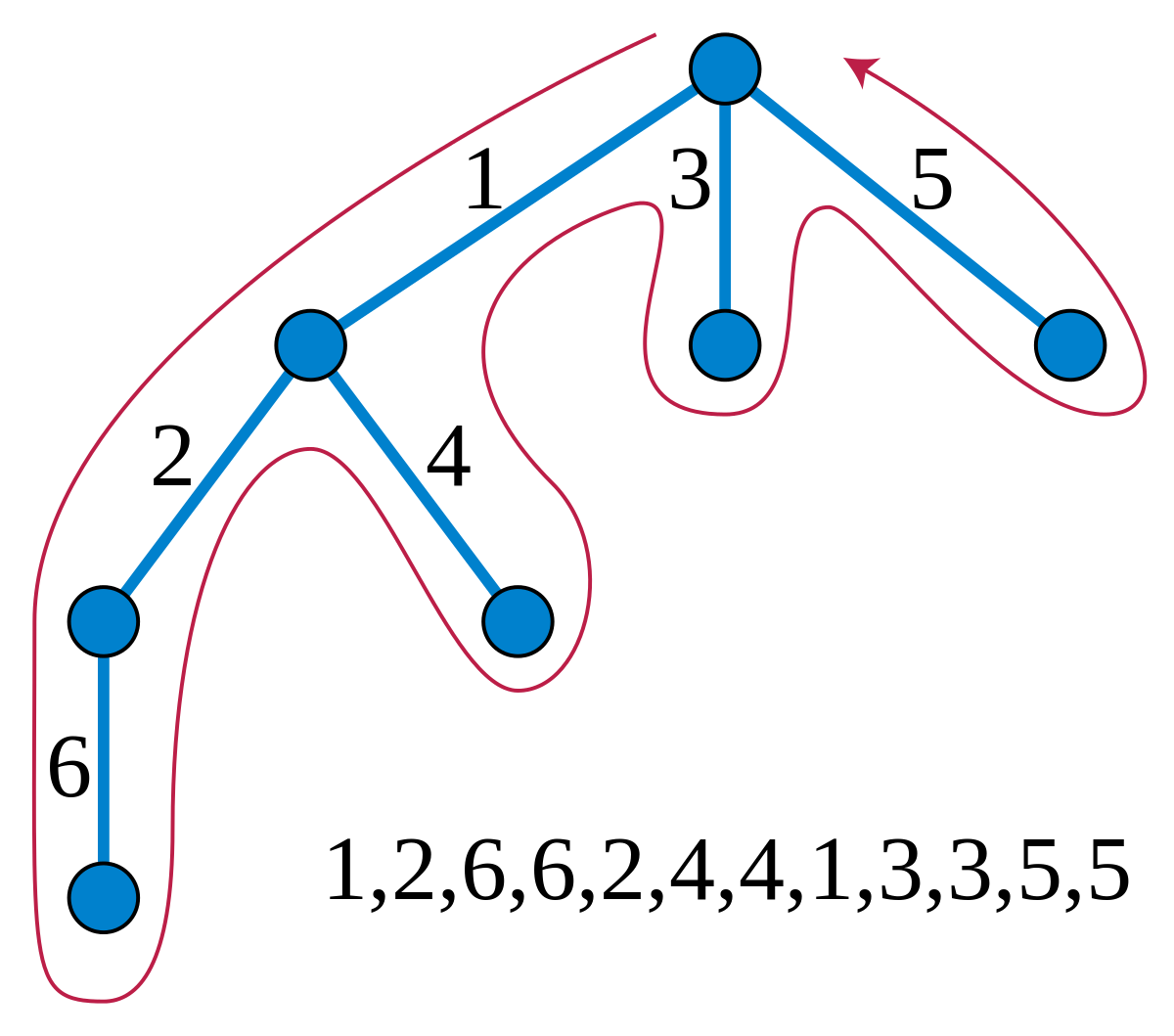
Fact: Given a tree $\mathcal{T}$ and $K$ paths on this tree, the union of these paths’ edges results in a subgraph with $O(K)$ nodes having a degree other than 2.
Proof of fact: Let Proceeding inductively, lets add the paths one by one to the subgraph, under the assumption that the subgraph takes the shape of a tree (if the end subgraph is a tree, then such a sequence must exist). Each path crosses the subgraph at most twice (otherwise there would be a cycle) by entering then leaving the subgraph. Thus all we do by adding the path is adding two branches to the tree. We leave the reader to formalise this into a proof.
 The virtual tree of black nodes is to the right
Applications: Given problems that involve paths on a tree, virtual tree lets us consider subsets of these paths in isolation in good time. Let us consider the following problem:
Problem: Given tree of $N$ nodes, answer $Q$ queries of the forms;
- Given a set of paths on this tree, deduce the diameter of the subgraph resulting from the union of these paths.
- Given a set of points on this tree, deduce the furtherest pair of points apart
The sum of the number of paths and points over all queries is $K$.
Solution: To Achieve $O((N+K)logN)$ complexity the problem reduces down really to building the virtual trees (forest) per query, compressing sequences of degree two “important” (not degree 2) nodes on the trees down to weighted paths, then finally running the standard diameter algorithm on the tree. Thus the problem boils down to constructing virtual trees efficiently. Now we discuss the construction of the virtual forest henceforth in 2 approaches.
Approach 1: for set of points
This elegantly applies LCA. Rooting the tree at 1, we note that any node which does not have degree 2 is the LCA of two of the nodes. We consider the following claim..
Lemma: Consider the nodes $v_1 … v_n$ in euler ordering (taking first occurrence of each label). Then for any $(x,y)$ there exist $z$ that $LCA(v_x,v_y)=LCA(v_z,v_{z+1})$.
Proof: Map the tree into an array of integers, where the index key is the position on euler ordering and index value is the depth of the node in that position. Then $v_l=LCA(v_x,v_y)$ corresponds to the node that is the result of $rangeminquery(pos(v_x), pos(v_y))$. Consider the nodes immediately to left and right of $v_l$ on the euler ordering. Then it follows that the LCA of these nodes is also $v_l$ by property of RMQ, as these nodes are necessarily enclosed by the interval $(pos(v_x), pos(v_y))$ as required.
Thus, we can effortlessly find the important nodes of the virtual tree, and it remains to link them up. We can do this by sweeping nodes by depth from high to low. Maintain a map keyed by euler order. When a node is encountered delete the nodes in the map contained by the interval it covers and set them as its children, being conscious of the edge lengths (take difference in depth). Then insert the node itself into the map.
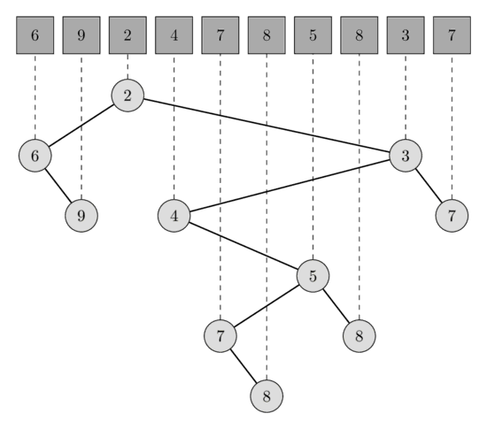
Turning Tree to RMQ
Approach 2: for set of paths
If we merely build the virtual tree for the set of path endpoints, then it must be that the actual virtual forest is a subset of the edges of this virtual tree. We simply must mark the edges which are relevant within this virtual tree. Thus we have the problem of being given the virtual tree of n nodes and calculating the union of paths on the tree in $\tilde{O}(n)$. Lets assume all paths go from ancestor (head) to descendant (tail) (otherwise split each path in two at the LCA). Euler traverse the tree, and when the head of a path is encountered insert the tail to a set that is keyed by euler tour. To decide whether an edge is on we merely have to check if there is an active node within the subtree of the edge. Now each path’s tail is only inserted and deleted once, so complexity is $O(nlogn)$.
The euler tour sweep
Lastly, it should we mentioned that the virtual tree is a good tool in module tasks to build up a tree as more information is obtained.
Greedy algorithms and small merge
Tree problems often involve greedy solutions, which are done through exploiting extremal structures in the tree such as the leaf. We discuss the following points:
- Solving the problem on subtrees
- Decrease and conquer (forced moves)
- Shaving off leaves
- The benefits of having a combinatorial upper/lower bound on the answer (Thanks Ray Li for teaching me this)
Example 1: Edge matching
Suppose that in a graph $G=(V,E)$ we want to find a max matching among edges where edges $u,v$ can be matched if they share a common endpoint (are incident).
We do this by constructing the edge tree through a dfs on the edges of the graph. In the resulting tree we observe two results:
- Every edge in the edge-dfs tree (henceforth edge-tree) corresponds to an edge in the original graph
- If two edges are incident in the edge-tree they are incident also in the original graph
We will now solve the edge-matching problem on this graph, and show that solving the problem on the tree.
Rooting arbitrarily, consider the deepest leaf $v$and its parent $p$. Suppose $p$ has no other children. Then we match the edges $(v,p)$ and $(p, par(p))$. Otherwise, we match $(v,p)$ with $(u,p)$ where $u$ is a sibling of $v$. This strategy, at every iteration, deletes two edges from the tree while maintaining the connectivity of the tree’s remaining edges. Thus with this strategy we can achieve $\lfloor \frac{E}{2} \rfloor$ matchings total, the theoretic maximum. Thus, as we can achieve the maximum by considering the tree structure, we can map this to a solution in the original graph.
This example shows us, that a naive upper bound, combined with consideration of subtrees, can reap rewards.
Resolving subtrees
Consider the problem Snap Tokens from ACIO 2021 Contest 2. While the actual problem asks for solutions on vortex graphs, we solve the problems on trees first.
Rooting the tree arbitrarily is a good start, and we should think about what happens in a subtree. We make a few observations:
- It should be obvious that an edge is traversed at most once, otherwise the two movements of tokens cancel out
- It should also be obvious that moving token $a$ to annihilate token $b$ is the same as moving $b$ to $a$
With this in mind, lets consider what happens in the subtree of $v$:
- If there is no tokens, we are done
- If there is one token, we are forced to move it upwards to the parent of $v$ (as moving tokens downwards to meet it is the same as moving it upwards to meet the token, so we should take care of the subtree)
- If we have multiple tokens in our subtree it gets interesting. We recursively solve the problem on the subtrees first, then some tokens would get moved to the node $v$. These cancel out, leaving nothing or at most 1 spare token behind. In the final case, we have to move this token upwards.
This gives us an immediate solution to the tree case, and by considering the vortex as trees hanging off a cycle, it turns out the problem is basically solved (the case of cycle left to reader).
However, a interesting extension to the problem is where there are updates of the form: Move a token from node $u$ to $v$ (we will concern ourselves with the tree case, the cycle is more tedious, but is largely uninteresting)
Now, we need a more elegant form of counting the number of needed moves. We apply some combinatorial thinking, and ask: Under what conditions do we need to move a token from $v$ to its parent (it is almost as if we try to lower bound the answer)?
We leave the reader to consider this. Note that even with this more elegant condition, HLD is needed to solve the problem.
Here, combinatorial thinking and breaking the problem into subtrees has paid dividends.
Job Scheduling (IOI19 practice contest)
This is a fantastic problem that I won’t spoil. But thinking about extreme “forced moves” within the decision making on the tree is a good course of action. This is also a valid approach for greedy problems in general.
Advanced DP on tree
DP on tree involves solving problems on subtrees of the original tree, then merging these answers to produce the original solution. However, there are many tools to accelerate these dps.
Optimising $O(N^2)$ to $O(NlogN)$
Suppose that a tree dp takes the form of $dp[\text{subtree v}][\text{some attribute j, say time}]$, but the transitions are relatively simple functions. Then we can use a data structure, like a segment tree or set, to maintain the second dimension $j$ for a subtree. We can use small merge to accelerate state transitions. Please see the section in “Segment Trees” on mergeable segment trees for an example.
Sibling dp
In short, an algorithm that appears to be $O(N^3)$ is actually $O(N^2)$. It is best explained with an example (courtesy of I_am_sb, from a Chinese Provincial Selection Exam)
The problem: Monochrome Tree You are given a weighted tree with $N\leq 2000$ nodes. You are also given an integer $0\leq K\leq N$. You are to choose $K$ nodes from this tree and colour them black, with the rest being coloured white. The score of the tree, which you must maximise, is the sum: \(S(\mathcal{T})=\sum_{u\ black} \sum_{v\ white} dist(u,v)\)
Output the maximium score. The solution: Rooting arbitarily and sing the most obvious dp state, we have $dp[i][j]=max$, where $i$ is the subtree, and $j$ is the number of black nodes assigned to the subtree. We apply our combinatorical thinking in constructinng our recursion, and think about the contribution of an edge to the final score.
Deleting a certain edge $(u,v)$ where $u$ is the parent of $v$, will say split the tree into two connected components with $x$ and $N-x$ nodes where $x$ is the size of the subtree at $v$. If we allot $b$ black nodes to the subtree of $v$ then $f(v,b)=b(N-x+b-K) + (K-b)(x-b)$ different black-white node pair paths will cross the edge $(u,v)$ , so the contribution of the edge $(u,v)$ is its weight multiplied by $f(v,b)$.
Let $slv(i)$ be a function that finds $dp[i][j]$ for all $0\leq j \leq size(i)$, where size denotes subtree size. Its psuedocode might look something like this, where we recursively solve the subtrees then do a knapsack dp to find the best allocation of black nodes to the subtrees.
void slv(v)
	Let c = num_children(v)
	Let dp2[size(v)][2] := new array
	for each child i = 1 ... c:
		Let s := sum of subtree sizes 1 ... i-1
		slv(i)
		for k = 0 ... size(i) // how many black nodes for i
			for j = 0 ... s:
				dp2[k+j][i%2] = max(dp2[k+j][i%2], dp2[j][(i+1)%2]+dp[i][k] + f(i,k) * W(v,i))
	dp[v][i] := dp2[i][c%2] FOR ALL i
On the surface the complexity seems terrible. But let us be a little more dilligent in our analysis.
Consider the following function, which is basically the same:
void disp(v):
	for each child i = 1 ... c:
		disp(v)
		for each node a in subtree of i:
			for each node b in subtrees 1 ... i-1:
				print(a,b)
Note that the complexity of the two functions disp and slv are same. Note further, that what disp does, is print every pair of nodes once, with disp(lca(a,b)) printing the pair (a,b). Thus we can also conclude that that slv() runs in $O(N^2)$, which solves our problem.
This is one of the more magical tree dps that can be used.
Note: By adding zero weight edges and nodes ignored in subtree size calculations, the implementation can be simplified by turning the tree into a binary tree. This is called the left-child right sibling idea, and is useful in these cases.
HLD and other data structures on Trees
Preorder Sweep and Euler Tour
Please see the page on segment trees.
HLD
Its useful and many other people can explain it better than I do. See cp-algorithms for a good explaination.
General Problems
- ACIO 2020 Open Contest Black Panthers
- ACIO 2020 Open Contest Vibe Check
- ACIO 2020 Contest 2 Tokens
- CEOI 2020 Spring cleaning
- CEOI 2019 Magic Tree
- Baltic OI 2015 Network
- Baltic OI 2020 Day 2 Village
- IOI 2019 Practice Contest Job Scheduling
- IOI 2018 Highway Tolls
- IOI 2013 Dream
- IOI 2011 Race
- IOI 2005 Riv
- COI18 Paprike
- FARIO 2011 Virus