RNN study notes
Recently I realised that I had never played with recurrent neural nets before and needed them for a task. So I spent the last few days learning them within the pytorch framework. Here are some brief notes I made. This is how I understand the concepts, and might not be entirely correct.
Concept of RNNs
Succinct diagrams of RNNs and the tasks they might be used for can be found here. It really is an exceptional reference.
In short, a RNN is a neural network module $f(x,h)$ that accepts a hidden state $h$ and a sequence $x_i$ and computes a new hidden state $h’$ and output $\hat y_i$. Can think of it as a fold operator on the input sequence $x_1 \ldots x_n$ and an initial hidden state $h_0$:
\[h_{i+1}, \hat{y}_{i} = f(x_i, h_i)\]or you can think of it as something of a neural Turing machine.
The RNN can be extended in multiple ways, such as multilayer (a.k.a deep) RNNs (the outputs of the first RNN is fed as input into the 2nd RNN), or bidrectional RNNs (where firstly an RNN takes sequence $x$ and generates sequence of embeddings $y$ going left to right, and a second RNN takes the embedding sequence $y$ and computes a s). See the above cheatsheet for more details.
Pytorch RNNs are very nice and handle the recurrent implementation automatically, along with adding dropout and multilayering.
Applications of RNNs
- Sequence classification (many to one): e.g sentiment classification
- Sequence to sequence (many to many): e.g translation (by encode decode architecture)
- Generative modelling (one to many): e.g language modelling by training RNN to model $p(x_n\mid x_1\ldots x_{n-1})$ and training to maximise the log likelihood of the training set
the first equality which holds by chain rule of conditional probability:
\[P(A,B,C)=P(A|B,C)P(B,C)=P(A|B,C)P(B|C)P(C)\]Training RNNs by Backproprogation through time (BPTT)
Let $L=L_1+\ldots +L_n$ be the total loss and $L_i=f(y_i,\hat{y}_i)$ be the loss on prediction $i$. The aim of any backproprogation algorithm is to compute
\[\frac{\partial L}{\partial W}\]where $W$ are the parameters of the neural network. In this case $W$’s parameters are applied $n$ times to $h_0$ to produce $h_{1\ldots n}$ from which $L_{1\ldots n}$ is derived.
In pytorch, autograd does all this for us so we just have to do the usual
optimizer.zero_grad()
optimizer = your_optimizer(rnn_model.parameters())
loss.backward()
optimizer.step()
and pytorch will do the rest.
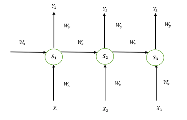
However there is aesthetically pleasing intepretation that comes in useful later . As the same parameters are applied repeatedly, we can “unfold” the network as below:

Where $S_i$ are copies of the original weights $W$ representing the $i$th application of the RNN to the state.
Then we can use chain rule
\[\frac{\partial L}{\partial W}=\sum \frac{\partial L}{\partial S_i}\frac{\partial S_i}{\partial W}=\sum \frac{\partial L}{\partial S_i}\text{id} = \sum \frac{\partial L}{\partial S_i}\]since $S_i$ are just copies of $W$ ($\frac{\partial L}{\partial S_i}$ is taken holding all other $S_i$ constant)
Training problems and solutions
Problem 1: Exploding and vanishing gradients
Neural networks are basically matrices with some nonlinearities and this analogy works even better if the nonlinearity is ReLU. So consider taking a matrix $A$ to power $k$. Now if $A$ has eigenvalues above 1 then $A^k$ will just blow up. And if all of $A$’s eigenvalues are below 1 the values will fizzle out. Due to the backproprogation algorithm being a lot like multiplying the same copy of a matrix if we proprogate through too many iterations, the gradients we compute will either vanish or blow up quite often which makes learning tricky (I think this is also why for deep neural networks sigmoid activation is not used in hidden layers, as the peak gradient of sigmoid is 0.25 which causes geometric decay in gradients)
Solution: Truncated BPTT and gradient clipping
One way we can try fix exploding gradients by just clamping gradients in a range. Pytorch has a function for this. But nevertheless backproprogating through so many iterations is very expensive.
Another solution is to use truncated BPTT. The idea is that the error $L_i$ of output $i$ should only have its gradients proprogated at most a certain distance. This ensures that the gradients proprogated are both meaningful and not too large, and also saves computational time.
This post has some good diagrams and indeed there are several ways to implement this idea. We will focus on the easier to implement method.
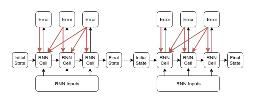
At a algorithmic level, what we are doing is the same as slicing the sequence up into blocks of size $k$, and treating each block as a independent data point except that we initialise the hidden state with the ‘summary’ state of the previous blocks like below:
 (taken from aforementioned blog post)
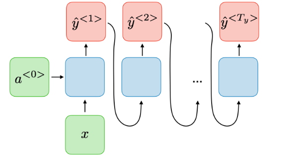
For simplicity lets assume here that the state passed between successive layers is the same as the output (see below)
 (taken from CS231 cheatsheet)
Then we can implement TBPTT in pytorch like:
optimizer.zero_grad()
loss.backward()
out = initial_out
for i in range(l):
    if i%trunc_size == 0:
        out = out.detach()
    loss += mLoss_fn(out, correct[i])
loss.backward()
optimizer.step()
The key to this is the .detach() function, returns a copy of out but with computational history cleared. It is also worthy to note that pytorch ‘persists’ past versions of a variable, say in this case out within its computational graphs for computing gradients, and this data is erased only when backproprogation is ran on the graph.
Problem 2: Capturing long term dependencies
Sometimes Sequences involve long term dependencies: For instance the bolded words below are seperated by great distance yet closely related.
I am chinese (insert 10000 words here) I speak mandarin.
Even though in theory RNNs can capture arbitarily long dependencies, in practice vanilla RNNs are pretty bad at doing this.
Solution: LSTMs
LSTMs (Long short term memory networks) are “improved RNNs” optimised for stable training (preventing memory issues). There are plenty of good articles like Chris Olah’s one here explaining it but the gist is that rather than passing 1 hidden layer between successive iterations, we pass 2 hidden states, the normal “hidden” layer and the new “cell” state instead. The “hidden” layer is now used to predict the next output, while the “cell” state is now used to persist data over longer distances, using gates to control the updating of information.
The pytorch implementation of LSTMs is quite nice and allows standard training tasks to be done very nicely so long as the sequences aren’t too long (in which case you’d need to use TBPTT).
Problem 3: Staying “on track”
Suppose we have a model whose output is repeatedly fed in as input again (see previous section for the diagram). If the model slips up once, it will most likely keep on slipping up and the rest of the output would be ruined. This would be very likely in the early stages of training process and hamper training efficiency.
Solution: Teacher forcing
We may use teacher forcing whenever some or all of the input (e.g recurrent state) to the $i$th iteration of the RNN is: (1) Available as ground truth or an direct encoding of ground truth (2) predicted by prior iterations of the RNN at inference (test) time For instance:
- A RNN is learning to execute an algorithm. The output of the $i-1$th step is then operated on by the RNN in the $i$th step (see neural algorithmic reasoning: the only difference there is that the problem scenarios are first encoded into high dimensional space and the recurrent ‘processor’ operates in that space)
- A RNN is converting a sequence of embeddings into a sentence (this happens in the encode-decode architecture of the language translation). The previous predicted word is fed alongside the current embedding position as well as previous hidden state to predict the next word (see this pytorch tutorial) in the sentence
The idea of teacher forcing is that we may substitute the part of the input which is generated by the RNN with the ‘true’ input: the ‘true’ input is given, the RNN is ran once on it and we can immediately provide feedback on this single step of the RNN by decoding the output and comparing with the target. For an example, if teacher forcing is used, it is often used for all steps of the example. And also note that if teacher forcing is used, there is no need to use BPTT (or TBPTT) since each time the RNN is only applied once.
The pytorch tutorial has example of this usage.
Teacher forcing greatly increases the 1-step accuracy of the RNN. However, it is advisable to only do teacher forcing on a example sometimes (say with certain probability $p$) as neural networks trained solely by teacher forcing are often less robust and more prone to multistep error.
General training tricks: DropOut
The aforementioned cheatsheet also contains a good list of tricks to optimising general NN performance. One of the ones I learnt about was DropOut. Dropout layers (nn.Dropout(p)) are placed after neural net layers. In short, what it does is that at train time with some probability $p$ the activations of each neuron in the layer before the dropout is set to 0. At test time (use model.eval() in torch), this is not done and instead the activations are rescaled accordingly to ensure the statistics of the activations remain same.
In short, the aim of dropOut is to force the neural network to have greater redundancy in its representation. This is as the training time zeroing of neuron activations forces the previous layer to express the same features in multiple ways as a single neuron can’t be relied upon to provide the correct activation. For an anology, in the real world, we check our math answers by doing the problem two different ways, and this is also what DropOut encourages in the neural net. It is generally found that neural nets trained with DropOut are more robust and perform better.
An Exercise: Learning to calculate prefix sums modulo $n$
I implemented some models and aformentioned techniques to get a sequence model to compute prefix sums modulo $n$. For example if $n=3$ then we’d need to map $[1,2,1]\to [1,1+2\equiv 0,1+2+1\equiv 1]$, so it is a sequence to sequence problem. We will work with $n=3$ throughout our experiment.
The numbers were encoded one-hot in a $1\times n$ tensor and the neural nets also output a softmaxed prediction (over $n$ classes) for the result.
We propose 2 models:
Model 1: LSTM with decoder (classical sequence to sequence) on the output. A small 0.1 dropout was used between the LSTM’s output and the decoder.
Model 2: We train an two layer NN taking in previous sum and current index value to compute new sum: i.e $f(Sum_{i-1}, val_i)\to Sum_i$
We train Model 1 with vanilla BPTT (i.e no truncation, no teacher forcing) and three different copies of Model 2 with teacher forcing (no BPTT needed), TBPTT and vanilla BPTT respectively to see what performed better. We also varied the length of training sequences (between 20 and 500) to see how training worked.
Findings
- Teacher forcing on model 2 worked very well. After all, teacher forcing on model 2 reduces the task to learning the modular addition operator, which is very easily done by a 2 layer neural network
- All models learnt to generalise with perfect accuracy when trained on length 20 sequences, even when teacher forcing was not used in model 2. We tested both architectures trained this way on length 5000 sequences and the accuracy was perfect.
- The models did not learn at all when trained purely on length 200 sequences. None of the models demonstrated test time accuracies on length 20 sequences of more than 35%. Truncated backproprogation did not seem to help either. This is suspected to because that the hidden states in later parts of the sequence are complete noise that we are effectively training models to predict the next sum when one of the required inputs (the hidden state in the case of LSTM or the previous sum $Sum_{i-1}$ for the second model) is complete noise
- This highlights importance of teacher forcing, as this is exactly the problem which it aims to fix, by giving the model ground truth instead of the previous predictions.
- This also highlights importance of training with some small simple examples, as our models learned well even without teacher forcing when the training sequences were small
The jupyter notebook is attached as pdf here.