Many discussions of variational autoencoders either present it in a intuitive view in terms of regularizing an ordinary autoencoder, or in a mathematical view, deriving it as a Bayesian latent variable model. I hope to reconcile the two views of the VAE in this discussion, first presenting it intuitively, then deriving it mathematically and showing the two views agree.
Intuitive View
Let us frame the discussion in the context of regular autoencoders. Recall that for normal autoencoders we have a encoder $f_\phi$ and decoder $g_\theta$ and try to minimize $|g_\theta(f_\phi(\textbf{x}))-\textbf{x}|^2$.
One might reasonably want to do the following things:
- semantically interpret the latent space (i.e what $f$ maps to)
- utilize the decoder to generate new samples by feeding in random points in the latent space
However, this is only possible if the latent projections satisfy:
continuity: points close together in latent space should correspond to ‘similar’ objects
completeness: Every point of the latent space, when decoded, should yield valid objects
With normal auto-encoders, this is not usually the case. Variational auto-encoders can be seen as applying noise regularization to solve this problem.
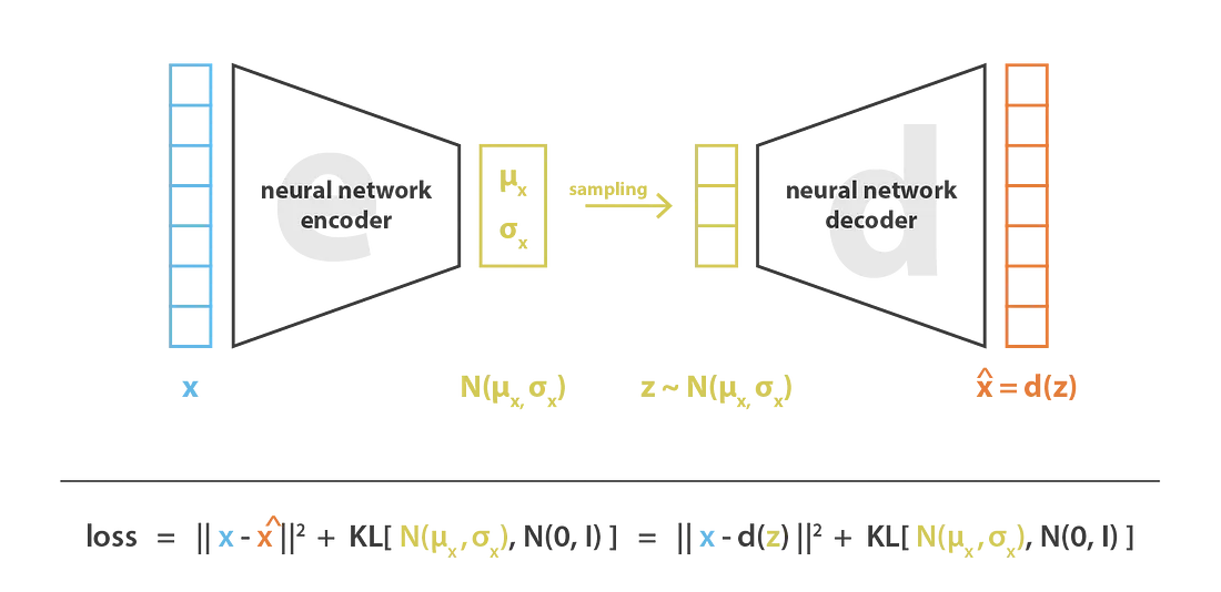
With variational autoencoders, we regularize by having $f_\phi(\textbf{x})$ map to a normal distribution (diagram taken from [1]):

- Take $\textbf{x}$, map it to $f_\phi(\textbf{x})\sim N(\mu_\phi(x), \sigma_\phi(x))$
- Sample $\textbf{z}\sim f_\phi(\textbf{x})$
- Decode $\textbf{z}$ as $\mathbf{\hat x}=g_\theta(\textbf{z})$
We train $\theta,\phi$ to minimize the following loss (here $\textbf{x}$ are datapoints): $\mathcal{L}=KL(f_\phi(\textbf{x}), N(0,I))+|\mathbf{\hat x}-\textbf{x}|^2$ (note $f_\phi(\textbf{x})$ is distribution so the equation makes sense)
Intuitively, two points of regularization are introduced:
- By feeding “noisy” versions of the encoding (by adding gaussian randomness), we try to encourage the model to group encodings of similar datapoints together in latent space (as we can see $\textbf{z}=\mu(x)+\sigma(x)\epsilon$ where $\epsilon\sim N(0,I)$)
- The second term of $\mathcal{L}$ is the familiar autoencoder reconstruction loss, whereas the first term regularizes the output distributions towards a standard normal distribution. This forces the $\mu$s predicted to be in “vicinity” of 0, thus ensuring the neighborhood of $\textbf{0}$ in the latent space contains only semantically meaningful vectors. It also forces the $\sigma$s to be nontrivial, thus which is necessary for the “noise” to have a meaningful regularizing effect.
Formal view
Setup
- We have a dataset $\mathcal{X}=\textbf{x}_{1}\ldots \textbf{x}_n$
- We assume that the data is sampled from a latent variable model:
- A latent variable $\textbf{z}$ is sampled from some prior $p(\textbf{z})$
- $\textbf{x}$ is sampled according to a posterior distribution $p(x\mid z)$
- This gives us both a Joint distribution $p(\textbf{x,z})$ and a distribution $p(\textbf{x})$ for $\textbf{x}$
- Our ultimate goal is for a given hypothesis space $\mathcal{P}$, find the best fitting distribution $p^*\in \mathcal{P}$ for the data (we will make this problem well defined & tractable by defining ‘best’ and the hypothesis space wisely)
Defining the Goal
- Define the hypothesis space to be the parametric family $\mathcal{P} = {p_\theta(\textbf{x,z})\mid \theta \in \mathbb{R}^n}$
- To define the family, in the spirit of the latent variable setup define
- $p_\theta(\textbf{z}) := N(0,\textbf{I})$ is fixed
- $p_\theta(\mathbf{x\mid z})$ is some parametrized function of $\textbf{z}$ (we will define it fully later)
- To define the family, in the spirit of the latent variable setup define
- The standard definition of ‘best’ when it comes to fitting distributions is to minimize the KL-divergence to the goal distribution i.e $KL(p_\theta | p)$ where $p$ is the true distribution
-
Optimizing KL-divergence from an empirical dataset is trying to maximize log likelihoods:
\[\max_{\theta} \sum_\chi \log p_{\theta} (\textbf{x}_i)\] -
However,
-
is intractable to estimate, let alone optimize against when $\textbf{z}$ is high-dimensional. - So we consider an related objective, the ELBO to maximize instead. This requires some new moving parts to be introduced
ELBO Loss
The key equation/result/definition is stated as follows:
Let $p,q$ be any two joint distributions on $\textbf{x,z}$ with suitable support, and write $p(\textbf{x}),q(\textbf{x})$ to denote the marginal distributions. Then for any fixed $\textbf{x}$,
\[\log p(\textbf{x}) = \mathcal{L}(\textbf{x},p,q)+D_{KL}(q(\textbf{z}\mid \textbf{x})\ \| \ p(\textbf{z}\mid \textbf{x}))\]where
\[\mathcal{L}(\textbf{x},p,q) := \mathbb{E}_{q(\mathbf{z\mid x})} [\log \frac{p(\textbf{x},\textbf{z})}{q(\textbf{z}\mid \textbf{x})}]\]is called the ELBO (Evidence Lower Bound) (note in above equation the randomness is in $\textbf{z}$)
Note that the name “lower bound” comes from the fact that $D_{KL}\geq 0$, which implies $\log p \geq \mathcal{L}$ for all $\textbf{x}$.
Applying ELBO
Recall that our grand objective is to find the best $\theta$ for our hypothesis $p_\theta$.
We further introduce the parametrized distribution $q_{\phi}(\textbf{z}\mid \textbf{x})$ as per definition of ELBO.
Then the ELBO is now a function of $\textbf{x}, \phi$ and $\theta$. Previously, we’d have liked to maximize log-likelihood, so we now content ourselves to maximizing the total ELBO
\[\max_{\theta, \phi} \sum \log ELBO(\textbf{x}_i,\phi, \theta)\]This allows us to finally define the learning procedure
- REPEAT:
- Let minibatch $\mathcal{B}={\textbf{x}_1\ldots \textbf{x}_k}$
- DO 1 gradient update step:
Now ELBO is intractable to compute exactly. However, we will now show that its gradient can be estimated from the definition by sampling for a given $\textbf{x}$.
Optimizing an expected value & reparameterization trick
We will approximate the gradient $\nabla_{\theta \text{ or } \phi} ELBO$ by random sampling, and then using it as if it was the ‘actual’ gradient.
Observe the distribution $q$ does not depend on $\theta$ so can just move the $\nabla_\theta$ inside the expectation to yield an estimator of $\nabla_\theta ELBO$. In particular, if we take $k$ samples $\textbf{z}^{(i)}$ then we can estimate:
\[\tilde{\nabla}_\theta ELBO(\textbf{x}; \theta, \phi)=\begin{align} \frac{1}{k}\sum_{i=1}^k {\nabla_\theta \log \frac{p_\theta(\textbf{x}, \mathbf{z^{(i)}})}{q_\lambda(\mathbf{z^{(i)}}\mid \textbf{x}).}} \text{, where } \mathbf{z^{(i)}} \sim q_\phi(\textbf{z}\mid \textbf{x}) \end{align}\]For $\nabla_\phi ELBO$ it is not so simple, as $q$ depends on $\theta$. One way we can go about things is via the REINFORCE (log-derivative) trick from reinforcement learning. This isn’t too bad but suffers in practice from high variance (the trick is stated clearly in [3])
Instead, we can first reparametrize (this is the reparameterization trick) $q$ by writing, $\mathbf{z\mid x} = T(\epsilon, f_\phi(\textbf{x}))$ where $\epsilon$ is a fixed random variable and $T$ is a deterministic transformation.
Often, the normal distribution is used, which gives us\(q(\textbf{z}\mid \textbf{x})=N(z\mid \mathbf{\mu}_\phi(\textbf{x}), \mathbf{\Sigma}_\phi(\textbf{x}))\) where $\mu,\Sigma$ are the two outputs of a neural network. Often $\Sigma$ is taken to be $\sigma_\phi(x)^2I$ for simplicity (and this works well in practice). In general, the original paper [0] states that any location-scale family suffices.
Then $\textbf{z} = \mu_\phi(x)+\sigma_\phi(x)\epsilon$ where $\epsilon\sim N(0,I)$
Then we can reframe the expectation with $\epsilon$ as the random variable to get
\[ELBO(\phi, \theta, \textbf{x}) = \int f(\epsilon) \frac{p(\textbf{x}, T(\epsilon, f_\phi(\textbf{x})))}{q(T(\epsilon, f_\phi(\textbf{x})), \textbf{x})}\ d\epsilon=\begin{align}= \mathbb{E}_{\epsilon} \left[\log \frac{p_\theta(\textbf{x}, T(\epsilon; \lambda))}{q_\lambda(T(\epsilon; \lambda))}\right] \end{align}\]and as the distribution is now independent of $\phi$ we can estimate the gradient $\nabla_\phi ELBO$ in same fashion as for $\theta$.
Recovering the intuition: Concrete realization of the VAE
We finally come back to defining $p(\mathbf{x\mid z})$. In the spirit of the reparameterization trick, we define \(p(\textbf{x}\mid \textbf{z}):=N(\mathbf{\mu}_\theta(\textbf{x}),I)\) as per [4] (the original paper demands that the variance is parametrized also by a neural network, but most implementations fix it to be $I$).
Calculations in original paper ([0]) gives an alternative expression for ELBO: \(\mathcal{L(\textbf{x},\theta,\phi)}=-D_{KL}(q_\phi(\textbf{z}\mid \textbf{x})\|p_\theta(\textbf{z}))+\mathbb{E}_{q_\phi(\textbf{z}\mid \textbf{x})}[\log p_\theta(\textbf{x}\mid \textbf{z})]\)
As $p$ has constant variance, we then have for some constant $C<0$,
\[\mathbb{E}_{q_\phi(\textbf{z}\mid \textbf{x})}[\log p_\theta(\textbf{x}\mid \textbf{z})]=C\mathbb{E}_{q_\phi(\textbf{z}\mid \textbf{x})}[\|\textbf{x}-\mu_\theta(\textbf{z})^2\|]\]which is akin to the reconstruction loss of ordinary autoencoders.
Thus maximizing $\mathcal{L}$ is equal to minimizing
\[D_{KL}(q_\phi(\textbf{z}\mid \textbf{x})\|p_\theta(\textbf{z}))+\beta\mathbb{E}_{q_\phi(\textbf{z}\mid \textbf{x})}[\|\textbf{x}-\mu_\theta(\textbf{z})^2\|]\]where $\beta=-C>0$.
And thus, we have recovered the loss function from the Intuition section where $q$ coincides with the encoder and $p$ the decoder. The overall procedure is thus simply to repeatedly estimate the gradients and take a step in the direction of the estimated gradient (which just corresponds to elbo_estimate.backwards() in pytorch).
Note: It is important that the KL divergence is analytically computable for the loss to be tractable to compute. However, when $p_\theta$ is a fixed Gaussian $N(0,I)$, the KL can be analytically computed (see [0] section 3 & appendices) to be \(\frac{1}{2}\sum_{j=1}^J (\mu_j^2+\sigma_j^2-1-\log(\sigma_j^2))\)where $\sigma_j,\mu_j$ are the variances and means of $q_\phi(\mathbf{z\mid x})$ (computed by each neural network) and $J$ is the size of the hidden dimension.
Addendum: Practicalities
We apply VAEs to the MNIST dataset
Experiment set-up
- A convolutional encoder & decoder was used (see code for architecture).
- I used someone else’s architecture in [5]
- As per the original paper we use mini-batch size 100 with $L=1$ samples per data-point, and a 2 dimensional latent space. Colab GPUs makes things a good deal faster.
- Adam optimizer with learning rate 0.001 was used, and the 60,000 MNIST examples in 600 batches were fed through the network 15 times (i.e 15 epochs)
- The encoder and decoder parameters were grouped into a single network for optimization
- Interestingly, when I tried to optimize encoder and decoder with 2 separate optimizers, things did not train as expected. Unsure whether bug or interesting phenomenon
Posterior collapse
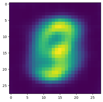
Variational autoencoders (VAEs) and other generative models often suffer from posterior collapse, which is a phenomenon in which the learned latent space becomes uninformative. For example, when trained with suboptimal hyper-parameters the VAE decoder learns to produce a single image regardless of the latent code.

This is likely due to the KL loss term providing excessive amounts of regularization, leading to over-smoothing of the data.
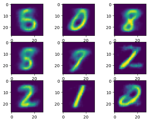
To tackle this issue, we vary the ratios of the reconstruction & KL loss components in the overall loss. I eventually settled on $0.01\times KL + \text{reconstruction}$. In the theoretical framework, this corresponds to setting $\beta = 100$.
This allows us to produce fairly convincing samples such as those shown below:

Fancier solutions such as described in [6] exist for this issue as well.
The colab jupyter notebook is attached as pdf here.
Main references
[0] Original paper: https://arxiv.org/pdf/1312.6114.pdf
[1] Good intuitive introduction: https://towardsdatascience.com/understanding-variational-autoencoders-vaes-f70510919f73
[2] Good discussion of mathematics underlying: https://deepgenerativemodels.github.io/notes/vae/
[3] The log derivative trick: https://andrewcharlesjones.github.io/journal/log-derivative.html
[4] Simplification: https://stats.stackexchange.com/questions/323568/help-understanding-reconstruction-loss-in-variational-autoencoder
[5] VAE architecture: https://github.com/r-gould/vae/blob/main/architectures/mnist.py
[6] $\beta$-schedule to prevent posterior collapse: https://medium.com/mlearning-ai/a-must-have-training-trick-for-vae-variational-autoencoder-d28ff53b0023